5 Practical Excel Tips to Work Smarter

5 Practical Excel Tips That Will Change the Way You Work

Whether you’re budgeting, tracking performance metrics, or just trying to make sense of a mess of data, Microsoft Excel remains an essential tool in any business toolkit. But unless you’re an excel expert, you’re likely only scratching the surface of what Excel can do. However, utilizing powerful functions and formulas can immediately speed up hours of manual organizations or calculations.

This guide walks you through 5 practical Excel tips and features that our accountants regularly use that are easy to learn, applicable in any industry, and improve your workflow. You don’t need to be a math genius or a programmer, just a willingness to learn a few foundational tools.

1. Flash Fill: Excel Learns Your Patterns

Our absolute favorite tip that can be useful for any situation, is just a click of a button, and doesn’t involve complicated formulas is Flash Fill.

Flash fill can automatically fill in values based on patterns you start to type, absolutely no formulas needed. For example, if you have one column that lists names as “Doe, John” but want them flipped to “John Doe”, all you need to do is type the correct formatting into an adjacent column, press ctrl + E and then excel fills in the rest.

This is one of the easiest, no-formula-needed excel tips that anyone from beginner to expert should be aware of because it can save hours of time spent reformatting. However, not every excel trick is this simple, but that doesn’t mean you can’t master them! We encourage you to open up excel and follow along to test out new tricks.

2. IF, AND, and OR: Let Excel Make Decisions for You

Before diving into any complicated formulas, it helps to get comfortable with Excel’s logic tools. The IF function in Excel is like giving your spreadsheet a brain: it helps Excel answer a yes-or-no question and returns different results based on the answer.

How it works:

The structure looks like this:

=IF(logical_test, value_if_true, value_if_false)

IF Example:

Imagine you’re checking if a temperature is at or below freezing (32°F) based on temperature data provided in column B. You can write:

=IF(B2<=32, “Freezing”, “Not Freezing”)

If the value in cell B2 is 30, Excel will return “Freezing.” If it’s 40, you’ll see “Not Freezing.”

What if there is more than one condition?

Want Excel to check two things at once? You can use AND or OR functions to articulate this.

• Use AND when both conditions must be true.
• Use OR when either condition can be true.

Example with AND:

Imagine you want to check if it is snowing, which is dependent on it being freezing and precipitating. You can utilize the formula you previously created, but then add to it based on the yes/no for precipitation in column C:

=IF(AND(C2=”Yes”, B2<=32), “Snow”, “Not Snow”)

Example with OR:

Now let’s say you want to identify ‘bad weather’, which you’ve determined is freezing (which we’ve already got a formula for) or excessively windy conditions based on wind speed being over 30mph. You don’t care which, and it could even be both, it just matters if either one is present. This is where OR comes in, used nearly identically to AND

=IF(OR(B2<=32, E2>30), “Bad Weather”, “Good Weather”)

These functions are essential for business rules, automated grading systems, eligibility checks, or task completion tracking. Plus, it’ll save you time from manually going through and writing it in yourself – especially helpful when you’re dealing with massive amounts of data.

3. SUMPRODUCT: Instantly Multiply and Add Rows of Data

Most people are familiar with the SUM and the PRODUCT function on their own, but did you know that you can combine them both into one function as an even more useful shortcut? It is particularly helpful when trying to calculate revenue, as you likely have multiple different products at multiple different price points. This function will multiply numbers in two or more columns row by row, then add each result.

Example:

Let’s say you’re calculating revenue for your fruit stands by multiplying quantity by price. Instead of calculating it all manually, use this formula:

=SUMPRODUCT(C2:C7, D2:D7)

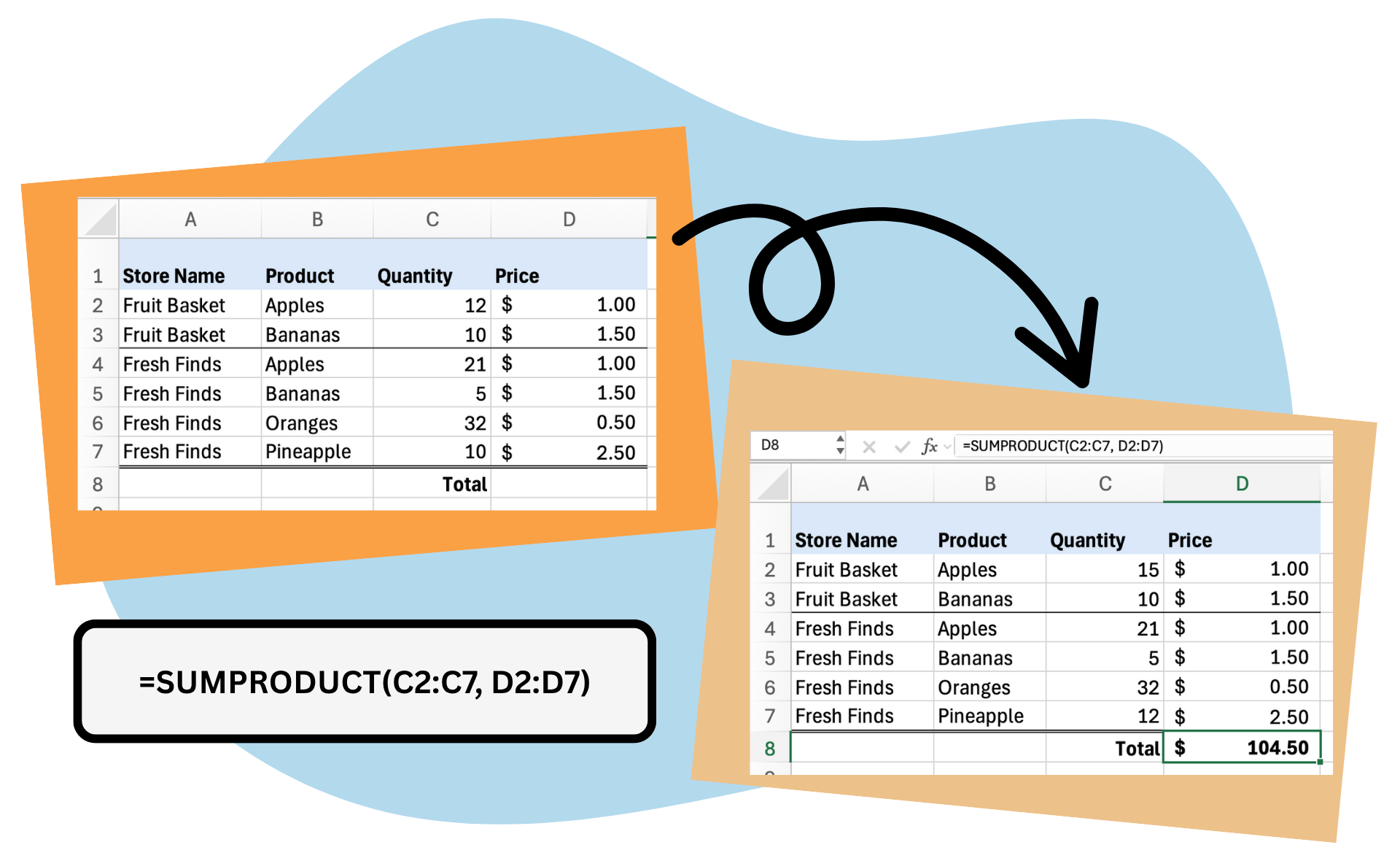
Pro Tip: You can even use filters during your formulas, so if for example you only wanted to know the revenue for Fruit Basket, you could use this formula:

=SUMPRODUCT((A2:A5=”Fruit Basket”)*C2:C5, D2:D5)

4. COUNTIF, SUMIF, and AVERAGEIF: Filter and Analyze Data by Criteria

You might begin to notice that several functions and formulas are combinations of the basic building blocks. So now that you understand IF functions, there are several functions that let you count, add or average numbers only when specific conditions are met using the IF function.

Let’s explore each of those, using this table as our example:

• COUNTIF: Counts how many times something appears. =COUNTIF(range, criteria)
  • Example: You want to know how many of your employees are female. You would use the formula: =COUNTIF(B2:B8, “female”)
• SUMIF: Adds values that meet a condition. =SUMIF(range, criteria, [sum_range]
  • Example: You want to add up total salary of all female employees. You would use the formula: =SUMIF(B2:B8, “female”, C2:C8)
• AVERAGEIF: Averages values that meet a condition. =AVERAGEIF(range, criteria, [averafe_range]
  • Example: you want to find the average salary of all female employees. You would us the formula: =AVERAGEIF(B2:B8, “female”, C2:C8)

Note that in both SUMIF and AVERAGEIF formulas you lead with the range for criteria, so you wouldn’t put whichever columns include salary first, as you won’t find the gender criteria in the salary column

As you can see from the example, this is especially useful when trying to find or summarize data based on certain demographics or categories, which is useful for HR, marketing, or budgeting.

5. SEARCH + IF(ISNUMBER()): Classify Text Automatically

When you’re working with text data in Excel—like customer feedback, product descriptions, campaign names, or survey results, you may run into a lot of text without an easy way to sort through them. But there is an easy way! You can automatically label or categorize entries based on certain words they contain by combining three functions: SEARCH, IF, and ISNUMBER.

SEARCH looks for a specific word or part of a word within a cell, then returns the position number of the first character where it finds that word. If the word is not found, it gives you an error. Because SEARCH returns a number only if the word is found, we can wrap it in ISNUMBER() to check if a match happened. Then, to top it all off, we can use the IF function to turn this into something meaningful by labeling it if a match happened.

So, let’s put it all together.

=IF(ISNUMBER(SEARCH(“text”, cell)), “name of identified cells”, “Other”)

Example:

Let’s say you several different files for marketing campaigns, and each year the naming convention changed. You want to to identify and categorize all campaigns that contain the word ‘display’. In column B, you enter this formula:

=IF(ISNUMBER(SEARCH(“Display”, A2)), “Display”, “Other”)

This is another great example of a tool that is especially helpful when sifting through massive datasets.

Conclusion

You don’t have to be an Excel expert to work smarter with your data. Just a few practical tools can make a big difference. These tips aren’t the flashiest or most complex, but they’re the ones our accountants rely on every day to save time, stay organized, and keep projects moving.

If you’re curious about how we can support you, please connect with us online, or reach out to us directly at 1-770-495-9077 or email us at [email protected].

The above article only intends to provide general financial information and is based on open-source facts, it is not designed to provide specific advice or recommendations for any individual. It does not give personalized tax, financial, or other business and professional advice. Before taking any form of action, you should consult a financial professional who understands your particular situation. CKH Group will not be held liable for any harm/errors/claims arising from the articles. Whilst every effort has been taken to ensure the accuracy of the contents, we will not be held accountable for any changes that are beyond our control.